Overview
Adaptation method
Description of our method for performing test-time adaptation.
Test-time signals
Examples of test-time signals that we employed.
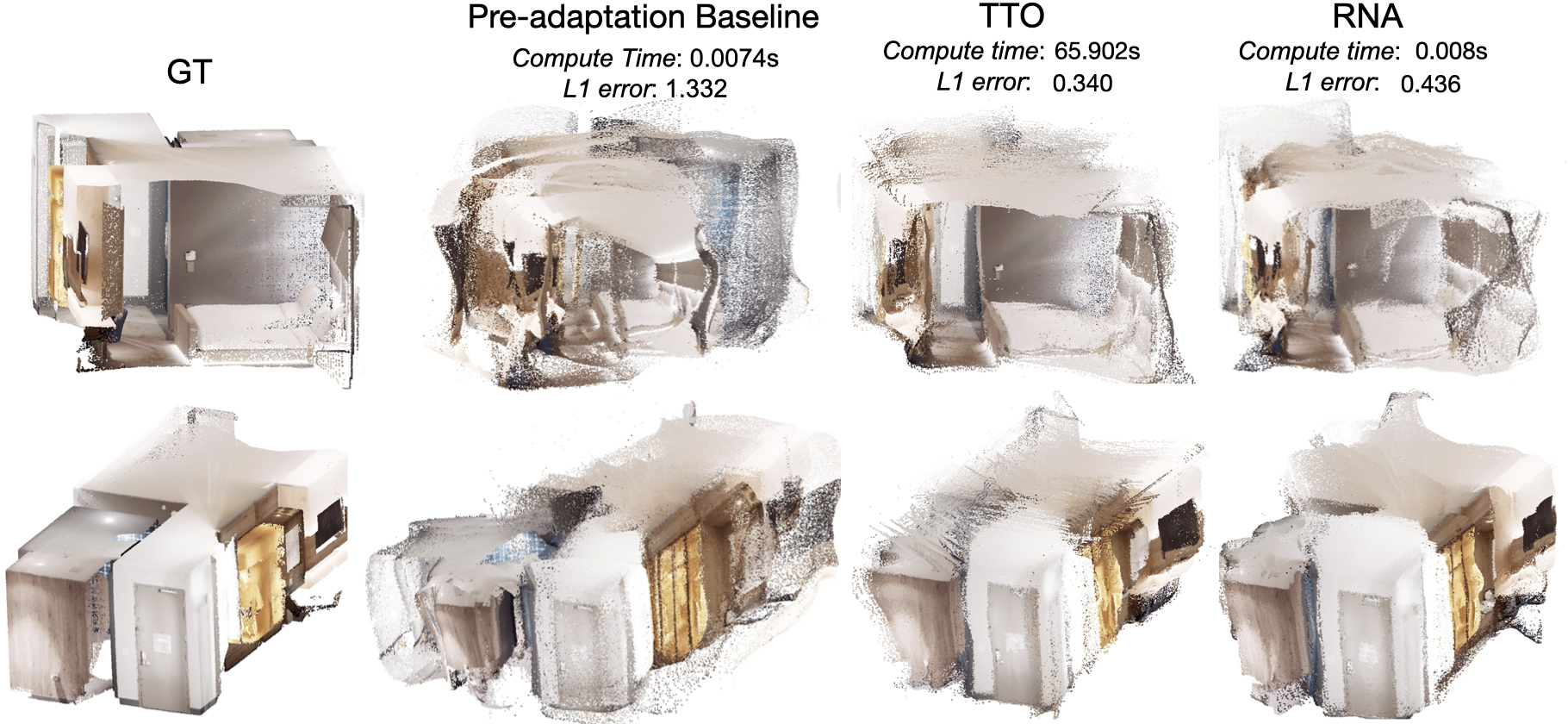
Sample results
Results on adaptation with RNA vs TTO and on different tasks.
Quick Summary
Neural networks are found to be unreliable against distribution shifts. Examples of such shifts include blur due to camera motion, object occlusions, changes in weather conditions and lighting. Dealing with such shifts is difficult as they are numerous and unpredictable. Therefore, training-time strategies that attempt to take anticipatory measures for every possible shift (e.g., augmenting the training data or changing the architecture with corresponding robustness inductive biases) have inherent limitations. This is the main motivation behind test-time adaptation methods, which instead aim to adapt to such shifts as they occur. In other words, these methods choose adaptation over anticipation. In this work, we propose a test-time adaptation framework that aims to perform an efficient adaptation of a main network using a feedback signal.
Adaptive vs non-adaptive neural network pipelines.
In order to be robust, non-adaptive methods include training-time interventions that anticipate and counter the distribution shifts that will occur at test-time (e.g., via data augmentation). Thus upon encountering an out-of-distribution input, its predictions may collapse.
Adaptive methods create a closed loop and use an adaptation signal at test-time. The adaptation signal is a quantity that can be computed at test-time from the environment. \(h_\phi\) acts as a "controller" by taking in an error feedback, computed from the adaptation signal and model predictions, to adapt \(f_\theta\) accordingly. It can be implemented as a (i) standard optimizer (e.g., using SGD) or (ii) neural network. The former is equivalent to test-time optimization (TTO), while the latter aims to amortize the optimization process, by training a controller network to adapt \(f_\theta\) - thus, it can be more efficient and flexible. In this work, we study the latter approach and show its efficiency and flexibility.
An adaptive system is one that can respond to changes in its environment. Concretely, it is a system that can acquire information to characterize such changes, e.g., via an adaptation signal that provides an error feedback, and make modifications that would result in a reduction of this error.
The methods for performing the adaptation of the system range from gradient-based updates, e.g. just using SGD to fine-tune the parameters (Sun et al.,Wang et al.,Gandelsman et al.), to the more efficient semi-amortized (Zintgraf et al.,Triantafillou et al.) and amortized approaches (Vinyals et al.,Oreshkin et al.,Requeima et al.). As amortization methods train a controller network to substitute the explicit optimization process, they only require forward passes at test-time. Thus, they are computationally efficient. Gradient-based approaches, e.g., TTO, can be powerful adaptation methods when the test-time signal is robust and well-suited for the task. However, they are inefficient and also have the risk of overfitting and the need for carefully tuned optimization hyperparameters (Boudiaf et al.). We will discuss this in more detail here. In this work, we focus on an amortization-based approach that we call Rapid Network Adaptation or RNA for short.
Below we show how we adapt a model \(f_\theta\). \(x\) is the input image, and \(f_\theta(x)\) the corresponding prediction. We first freeze the parameters of \(f_\theta\) and insert several FiLM layers into \(f_\theta\). We then train \(h_\phi\) to take in \(z\), the adaptation signal, and \(f_\theta(x)\) to predict the parameters of these FiLM layers. This results in an adapted model \(f_{\hat{\theta}}\) and the improved predictions, \(f_{\hat{\theta}}(x)\). We will show that adaptation with \(h_\phi\) results in a closed loop system that is flexible and is able to generalize to unseen shifts.
Architecture of RNA.
While developing adaptation signals is not the main focus of this study and is independent of the RNA method, we still need to choose some for experimentation.
Existing test-time adaptation signals, or proxies, in the literature include prediction entropy (Wang et al.), spatial autoencoding (Gandelsman et al.) and self-supervised tasks like rotation prediction (Sun et al.), contrastive (Liu et al.) or clustering (Boudiaf et al.) objectives.
The more aligned the adaptation signal is to target task, the better the performance on the target task (Sun et al., Liu et al.). More importantly, a poor signal can cause the adaptation to fail silently (Boudiaf et al.,Gandelsman et al.).
The plot below shows how the original loss on the target task changes as different proxy losses from the literature, i.e. entropy, consistency between different middle domains are minimized.
In all cases, the proxy loss decreases, however, the improvement in the target loss varies. Thus, successful optimization of existing proxy losses does not necessarily lead to better performance on the target task.
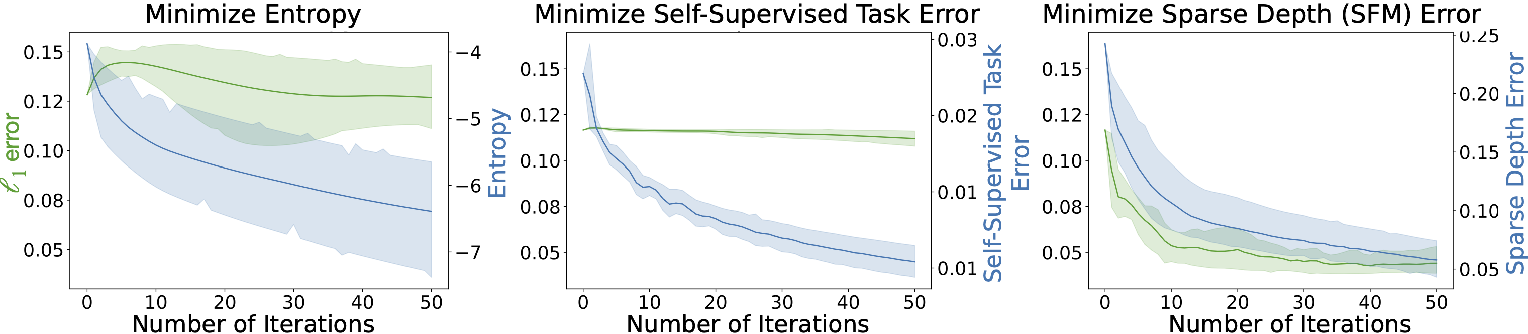
Adaptation using different signals. Not all improvements in proxy loss translates into improving the target task's performance. We show the results of adapting a pre-trained depth estimation model to a defocus blur corruption by optimizing different adaptation signals: prediction entropy, a self-supervised task (sobel edge prediction error), and sparse depth obtained from SFM. The plots show how the \(\ell_1\) target error with respect to ground-truth depth (green, left axis) changes as the proxy losses (blue, right axis) are optimized (shaded regions represent the 95% confidence intervals across multiple runs of SGD with different learning rates). Only adaptation with the sparse depth (SFM) proxy leads to a reduction of the target error. This signifies the importance of employing proper signals in an adaptation framework.
We show some examples of test-time adaptation signals for several geometric and semantic tasks below. Our focus is not on providing an extensive list of adaptation signals, but rather on using practical ones for experimenting with RNA as well as demonstrating the benefits of using signals that are rooted in the known structure of the world and the task in hand. For example, geometric computer vision tasks naturally follow the multi-view geometry constraints, thus making that a proper candidate for approximating the test-time error, and consequently, an informative adaptation signal.

Examples of employed test-time adaptation signals. We use a range of adaptation signals in our experiments. These are practical to obtain and yield better performance compared to other proxies. In the left plot, for depth and optical flow estimation, we use sparse depth and optical flow via SFM. In the middle, for classification, for each test image, we perform \(k\)-NN retrieval to get \(k\) training images. Each of these retrieved image has a one hot label associated with it, thus, combining them gives us a coarse label that we use as our adaptation signal. Finally, for semantic segmentation, after performing \(k\)-NN as we did for classification, we get a pseudo-labelled segmentation mask for each of these images. The features for each patch in the test image and the retrieved images are matched. The top matches are used as sparse supervision.
To perform adaptation at test-time, we first compute the adaptation signal as described above. The computed signal and the prediction from the model before adaptation, \(f_\theta\), are concatenated to form the error feedback. This error feedback is then passed as inputs to \(h_\phi\) (see the figure here). These adaptation signals are practical for real-world use but they are also imperfect i.e., the sparse depth points do not correspond to the ground truth values. Thus, to perform controlled experiments and separate the performance of RNA and adaptation signals, we also provide experiments using ideal adaptation signals, e.g., masked ground truth. In the real world, these ideal signals can come from sensors like Radar.